Segmented Spot Size Converter (GA + 3D BPM)

1.5% Δ silica channel waveguide (5×5 µm) ↔ SMF at 1301 nm — segment width/gap optimized with a genetic algorithm driving a 3D BPM loss evaluation.

Target & SMF parameters

Wavelength (µm) SMF MFD (µm) WG width W (µm) WG height H (µm) Δ (%) Expanded MFD (SSC out) (µm)

The last field is the mode-field diameter the SSC tip presents to the SMF (a design target the GA searches for). Set it equal to the bare WG MFD to see the loss without a converter.

n_core (from Δ)

—

n_clad (silica, Sellmeier)

—

Bare WG mode field diameter (D4σ)

—

Coupling loss — bare WG ↔ SMF

—

Coupling loss — SSC tip ↔ SMF

—

Improvement

—

SSC quality

—

Gaussian–Gaussian overlap model for a quick estimate; the real design objective is the 3D-BPM output power below.

Mode field cross-section — blue: SMF Gaussian, red dashed: bare WG mode, green: expanded SSC-tip mode. Larger overlap with the SMF means lower loss.

Why a spot size converter

The SMF mode-field diameter is ~9.2 µm at 1310 nm, while a 1.5% Δ, 5×5 µm silica waveguide guides a much smaller mode — the mode-size mismatch is the dominant butt-coupling loss.
Expanding the waveguide-end spot to approach the SMF mode maximizes the overlap integral and cuts the loss.
A segmented (periodically broken) taper uses sub-/near-wavelength duty modulation to lower the local effective index gradually, expanding the mode adiabatically in a shorter length than a plain linear taper — and it respects mask minimum-linewidth rules.
Target: SMF coupling insertion loss < 0.3 dB, with polarization and wavelength insensitivity.

Structure & design variables

The segment list is generated from a small parameter vector; the GA treats that vector as the gene.

Variable	Meaning	Search range (example)
`W1`	Segment start width (SMF side, wide)	6.0 – 9.0 µm
`W2`	Segment end width (waveguide side)	4.0 – 5.0 µm
`ΔL`	Segment period (pitch)	3 – 8 µm
`P1 / P2 / P3`	Per-section duty (fill / period)	0.1 – 0.9
`L0 / L1 / L2`	Input / 1st / 2nd taper section lengths	50 – 200 µm
`L3 / L4`	Connecting taper / output waveguide length	20 – 80 µm

Duty violating the mask minimum linewidth / gap (e.g. 0.5 µm) is clipped or penalized in the fitness function.

Optimization workflow (GA ⇄ 3D BPM)

① gene → structure: the parameter vector builds the segment list (begin.z, width, duty) and writes silica_line_seg.ind.
② 3D BPM run: launch the SMF mode, propagate, read the output-monitor power (overlap with the waveguide mode).
③ fitness: Loss = −10·log10(P_out) [dB]; the GA minimizes loss. Average over polarization (TE/TM) and wavelength (1290/1301/1310 nm) for robustness.
④ select · cross · mutate: tournament selection + real-coded crossover (BLX-α / SBX) + Gaussian mutation; constraint violations penalized.
⑤ iterate: stop when the best loss stalls for K generations.

Objective: minimize f(g) = mean_{λ, pol} [ −10·log₁₀ P_out(g) ] + penalty(g)

% Fitness (MATLAB pseudocode) — extend the existing seg_ssc_.m
function loss = eval_ssc(gene)
    write_ind(gene);                       % (1) gene -> .ind
    dos('start /w bsimw32 silica_line_seg.ind prefix=seg_ wait=1');  % (2) 3D BPM
    P    = read_last_power('seg_.mon');    % output power (overlap)
    loss = -10*log10(P);                   % (3) dB, smaller is better
    loss = loss + penalty(gene);           % min-linewidth / gap penalty
end

% GA driver
%   ga(@eval_ssc, nvars, [], [], [], [], lb, ub, @constraints)
%   (MATLAB Global Optimization Toolbox) or a custom GA loop.
%   BPM is expensive -> evaluate the population in parallel (multiple prefixes),
%   or use a surrogate (Kriging) to cut BPM calls.

GA optimization result @ 1301 nm

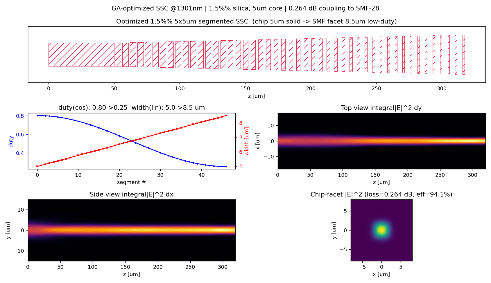
A pure-Python pipeline (gdstk segment generation → self-written split-step 3D BPM → genetic algorithm) was run for the target spec: chip waveguide 5 µm × 5 µm solid on the left, 8.5 µm-wide low-duty SMF facet on the right, thickness fixed at 5 µm. The GA freely tuned the pitch, number of segments, and the duty / width ramps.

Quantity	Optimized value
Coupling loss @ 1301 nm (fine grid, dx = 0.15 µm)	0.264 dB (η = 94.1 %)
Pitch / number of segments	5.73 µm / 47
Duty ramp (start → end)	0.80 → 0.25 (cosine profile)
Width ramp (start → end)	5.0 → 8.5 µm (linear)
Total device length	319 µm
Residual (non-radiated) power	0.977

The narrow solid end is a well-guided chip mode (3.1 µm); toward the wide low-duty end the sub-wavelength segments lower the effective index so the mode expands to ≈ 12.7 × 10.9 µm and matches the SMF-28 mode field (9.2 µm). Launch is done at the SMF facet and overlapped with the chip mode at the opposite facet (reciprocity ⇒ same as chip→SMF).

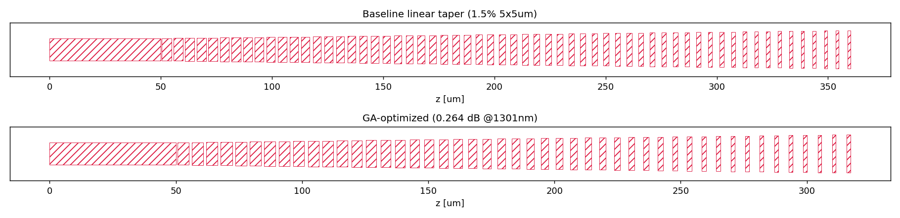
GA-optimized SSC: geometry, duty/width ramp, top/side BPM field, and chip-facet output mode — GA-optimized SSC — geometry, duty/width ramps, top & side |E|² propagation, and the clean single-mode chip-facet output.

Uploaded reference segmented SSC vs GA-optimized — Baseline linear taper vs. the GA-optimized geometry (0.264 dB on the fine grid).

Downloads

Everything needed to reproduce the result above:

ssc_optimized.gds — GA-optimized mask layout (47 tapered segments, chip 5 µm → SMF facet 8.5 µm).
ssc_reference.gds — the reference segmented SSC layout for comparison.
seg_ssc.py — segmented-SSC generator, 3D-BPM index field, evaluator, and the GA optimizer.
ssc_ga_optimizer.py — platform constants (1301 nm silica Sellmeier), 3D-BPM evaluation, and the continuous-taper GA base.
run_seg_ga.py — driver that fixes chip width = 5 µm / SMF-facet width = 8.5 µm (1.5% Δ, 5 µm core) and runs the GA.
ssc_result_summary.png — full result figure.
ssc_compare.png — reference vs. optimized comparison figure.

Run with python3 run_seg_ga.py (needs numpy, gdstk, and bpm3d.py). Add --fast for a coarse-grid search; always re-validate the final candidate on the fine grid (dx ≤ 0.15 µm, window ≥ ±18 µm).

1.5% 5 µm × 5 µm SSC